
本文作者:旅菇佘侨159
本文分类:系统与软件 编程学习笔记 计算机技术 浏览:2005
阅读时间:9137字, 约10-15分钟
Introduction
It is a commonplace practice to estimate, evaluate, and compare the educational qualities of middle schools by using an enrollment based metric. To elaborate, if one intends to measure the quality of a school, he or she will calculate the proportion of students there that are accepted into prestegious high schools. A school is defined as superior if it can ensure a greater ratio of Quality High School Acceptance. For example, at Huayu Middle School in Xuhui District, Shanghai, more than one third of the students are ultimately accepted into Shanghai High School , the best of the renowned "Four High Schools" in Shanghai, each year. In addition, another 50 students or so will find their way into the other three good schools, or into Qibao High School, another educational powerhouse. Altogether, this data enshrines Huayu as practically the best middle school in all of Shanghai.
Despite being effective and straightfoward, this acceptance rate metric has its shortcomings. It is a Frequentist measurement that assumes the likelihood as an approximation of the prior probability. Plainly speaking, a Huayu student may regard the historical acceptance frequency (likelihood) as the acceptance probability (prior) for himself/herself, which is far from reality. Hence, this model is ,to a certain extent, deceptive, for it conceals and disguises our ignorance on the topic. Note that if "Big data" is present in this context, then the Frequentist assumption will stand well. If so, one can then happily use the likelihood as the approximate prior probability. Unfortunately, with the amount of data present ,uncertainty is not, and cannot be completely eliminated from the scope. Therefore, I would like to present to you ,in this blog post, a Bayesian approach to the issue of evaluating middle schools.

An Introduction to Bayesian Inference
Bayesian methods are one of many in a modern data scientist's toolkit. They can be used to solve problems in prediction, classification, spam detection, ranking, inference, and many other tasks.
—— Bayesian Methods for Hackers
The philosophy of Bayesian Inference is very simple. It involves updating your beliefs after considering new evidence, which is natural to us humans. If one keeps making mistakes on a certain kind of problem, then he will start to lose confidence in his ability to solve this particular sort of problem. Conversely, if one seldom fails to do some kind of problem, his confidence will grow. Though, he will never be absolutely sure in himself. Bayesian Inference works identically: We update our beliefs about an outcome, but rarely can we be absolutely sure unless we rule out all other alternatives.
From the Bayesian Perspective, probability is interpreted as measure of believability. That is, how confident we are in an event occuring. If we assign an event with the probability 0, then we are asserting our belief that this event will never happen. Assigning 1, on the other hand, asserts something that is bound to happen. Assigning a value in between will mean that the event would have some chance of happening, but we are not totally confident.
The belief we hold on a certain event before seeing any evidence is called a prior. It reflects our intuitive thought on an issue, and it is potentially very wrong. For example, if you are presented with a dice, then you might assume that it is unweighted, having a uniform distribution of probability across its six sides. Then, the evidence from experimentation and observation that help us update our beliefs is called the likelihood. E.g. you roll the dice six times and find that you get "6" three times, "4" twice, and "2" once. Finally, you update your prior according to the likelihood, and obtain a more accurate belief about the event, namely, the posterior. The method of update can vary. A typical method might be MCMC (Monte Carlo Markov Chain), which applies a method dubbed rejection sampling to intelligently explore the posterior landscape, returning an amount of samples cumulatively called a trace. A more state-of-the-art sampler would be the No-U-Turn-Sampler, or NUTS. NUTS belongs to the HMC (Hamiltonian Monte Carlo) family of samplers, which utilizes the gradient of the posterior landscape to assist the sampling process. This would sound quite familiar to Neural Network enthusiasts, who uses Tensorflow or Pytorch in their work very often. To me, though, the intuition behind HMC is more straightforward: the posterior is really regarded as a “landscape”, complete with notions of gravity! The sampler can then be seen as an infinitesimal ball traversing it, governed by kinetic and potential energy…… The details of these go beyond this article: those of you interested can look it up yourself.

In the dice example here, however, a very neat mathematical trick can be used, which allows us to directly express the posterior distribution in its exact form! This trick is called using a Conjugate Prior. The conjugate prior of the Binomial Distribution is called the Beta Distribution, while the conjugate prior of the Multinomial Distribution is called the Dirichlet Distribution. How do we use the conjugate prior to derive the posterior? The dice conforms to a multinomial distribution with 6 outcomes. Hence, it has a Dirichlet conjugate prior with 6 parameters. The uniform prior of probabilities(p = {0.167 * 6}) we assigned to the dice can be put down as p ~ D(θ),where θ = {1,1,1,1,1,1}. How do we add the likelihood into it? Simply add it with the parameters! Now we have p ~ D(θ') where θ' = θ + Δθ, Δθ={3, 0, 2, 0, 1, 0}. θ' = {4, 1, 3, 1, 2, 1}. This method will be used in the discussion of admission rates below.
Inference of the True Acceptance Rate
We shall commence the modelling of High School Enrollment from a Bayesian perspective. The true acceptance rate for each of the Four High Schools is the unknown variable ->p, with five possible outcomes: SHS, EFZ, FF, JF, and None. We choose the Dirichlet Multinomial D as the prior distribution of ->p.
There is no official, centralized and recognized source for the enrollment data of each school. Thus, we adopt the data from https://zhuanlan.zhihu.com/p/160201890.
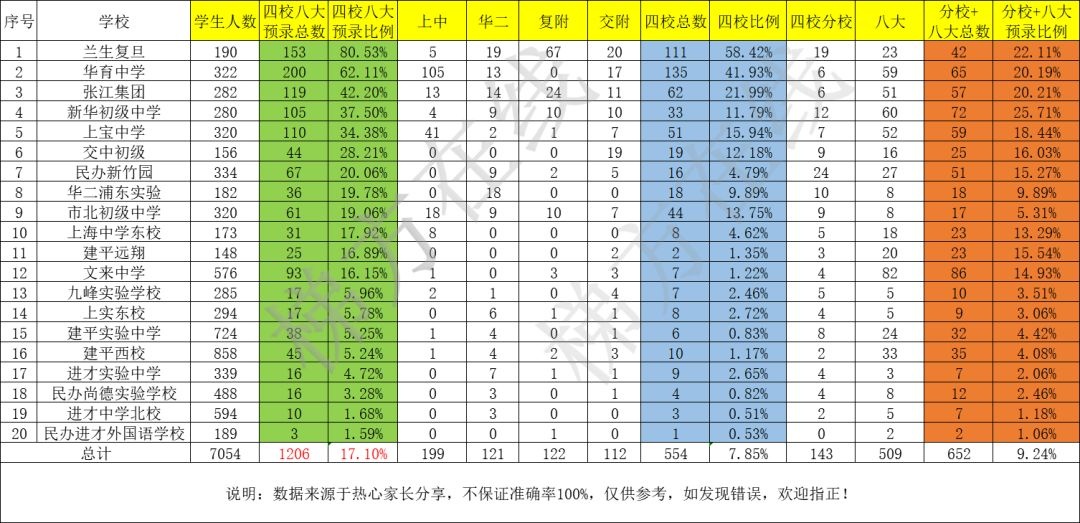
Note that I was only able to obtain the data via Preemptive Enrollment. Technically the enrollment via admission test should be included as well, but that's a nebulous administrative allocation even harder to obtain.
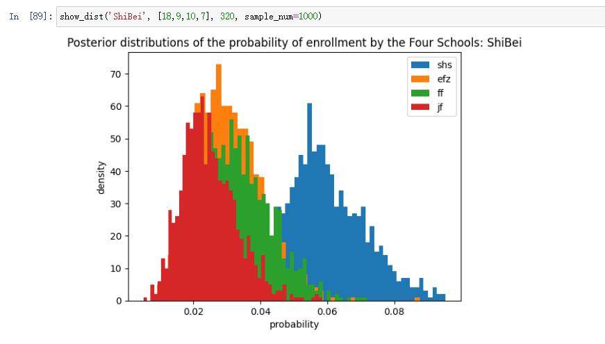
We assume the Uniform Prior for each school. For each student, a five-sided "dice" is cast. Here we try to determine how the dice is weighted for each school.


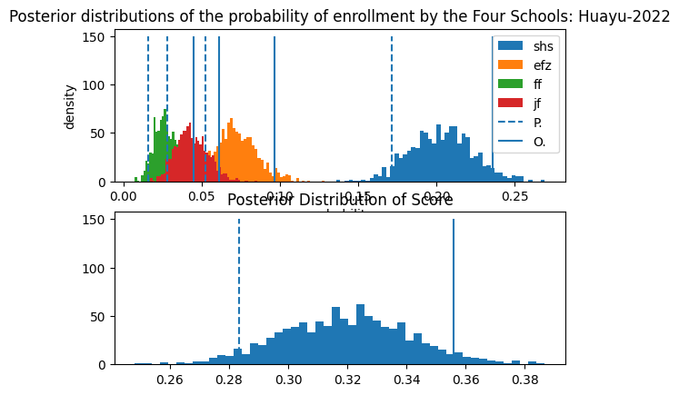
These are the shapes of the posterior distributions. The Dirichlet is sometimes called the "Distribution of Distributions", because it actually contains probability vectors that can dictate the shape of a whole family of distributions. Here the distribution for None is not displayed, as it generally takes much greater values than actual enrollment. Note that the five probabilities should sum up to 1 in each individual sample.
From the posterior densities, we can infer that Huayu students have a 30% to 35% chance of entering SHS through Preemptive, but only around 5% for JFZ and EFZ, and around 0% for FF. For a Lansheng student, the worst-case-scenario still offers a more than a 30% probability to enter FF, while the best-case-scenario approximates 50%! (Are we talking about die or coins?) Notice that the distributions for Lansheng are spread out more than those from Huayu. That is, they have a larger variance. This is a result of Lansheng's smaller size, which puts more doubt on the posterior. In other words, with only 190 samples, Lansheng's data eliminates less uncertainty from the prior. This is one of the beauties of Bayesian Inference, where uncertainty is retained, and a more robust comparision can be done between entities of varying size.
Evidently the SHS is inclined towards Huayu, while FF is inclined to the Lansheng Fudan, a well know phenomena.
Here are some other schools.
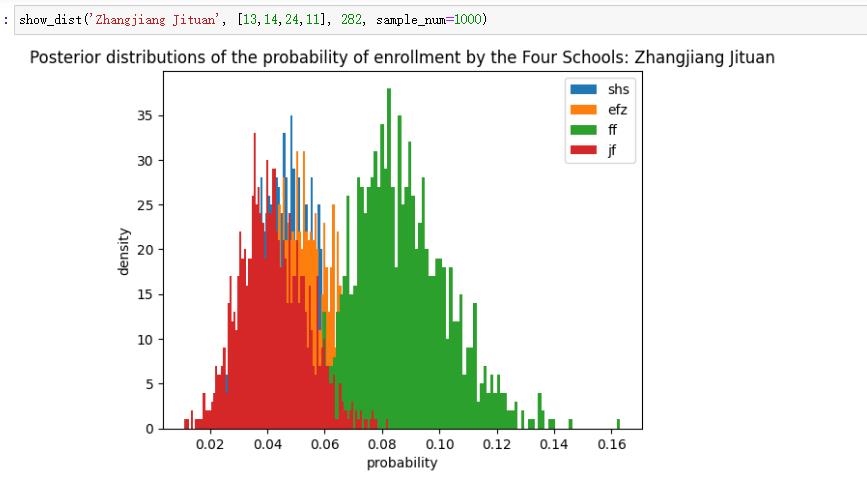

Note the difference in scale for the axes.
Applying a Loss (Win) Function and CI
"Staticians are a sour bunch. They measure the outcomes in terms of Losses. When one wons, he or she says that he or she Lost Less"
Bayesian Inference for Hackers
Now we have estimated the distribution of enrollment probabilities, we should summarize them in a robust way. It is said that SHS and EFZ are the better two of the Four Schools, because more of their students are further admitted into Tsinghua or Peking University, while FF and JF students primarily go to Fudan and Jiaotong University. Actually this layer of admission can also be modelled with a Dirichlet-Multinomial. But I did not wish to create something resembing a Latent Dirichlet Allocation just yet. So I simply assigned the Win score 1 to anyone going to SHS or EFZ, and 0.6 to anyone going to FF or JF.
Aside from this "Win Function", I decided to mark the CI (Confidence Interval) as well. If a scenario of admission is so bad that only 5% percent of the simulated scenarios are worse, then we call it the 5% lower bound. Conversly, a super win situation that is better than 95% of the simulated situations is deemed the 95% upper bound. We mark the two limits with lines.
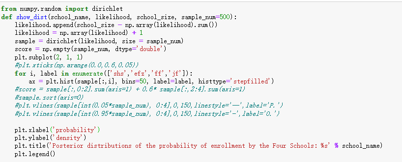
Here's the revised code:
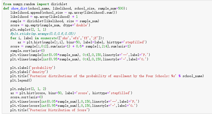
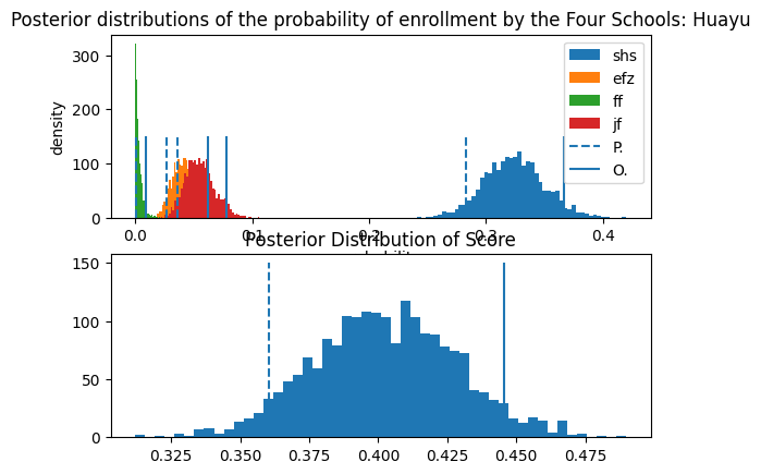
In the legend, P. and O. stand for Pessimistic and Optimistic.

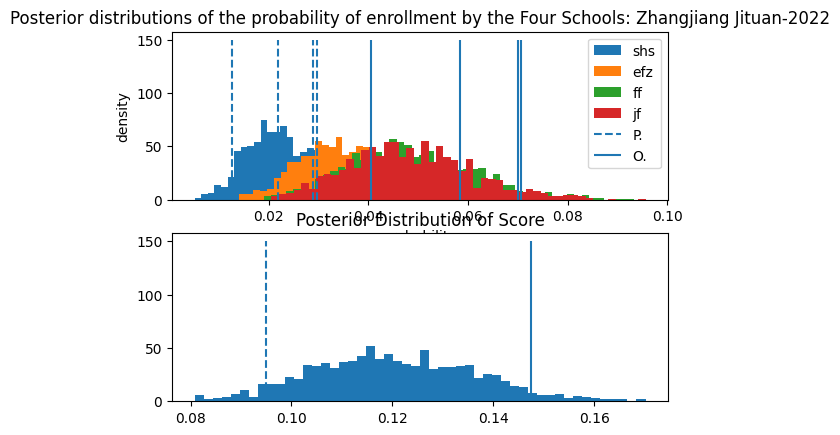
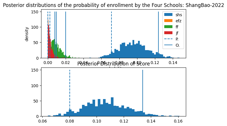

We also have another Evaluation of Huayu with 2022 Data.
Here are some numeric summaries :
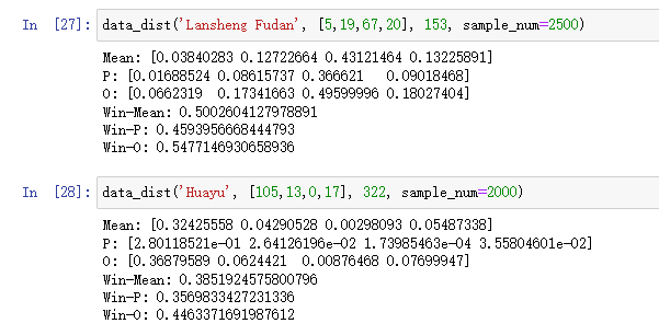
It appears that in the year 2020, Lansheng beat Huayu in terms of Preemptive Admission. However, we have to consider a large amount of Huayu Students still manage to enter SHS through the Standardized Test, the data of which I was not able to obtain. Furthermore, if the coefficent of FF and JF is lowered to 0.4 from 0.6, the win distribution of Lansheng does not significantly excel that of Huayu.
Summary
In this blog post, I experimented with infering the posterior admission rate of various middle schools in Shanghai using Bayesian Statistics. I intend to propose an alternative to the Frequentist admission-based-metric for evaluating Chinese Schools. In this model, we can quantify the uncertainty of the values, instead of having just one mean value. Comparing Schools in this perspective is simply calculating the probability that one excels another in the designated norm, namely the "Win function". We can also compare according to the Worst-Case-Scenarios, where the enrollment of the school is at the theoretical worst.
Anglo-Chinese Cross Reference of Technical Terms
Bayesian Inference: 贝叶斯推断
Prior, Likelihood, Posterior: 先验、似然、后验
Conjugate Prior: 共轭先验
Binomial Distribution: 二项分布
Multinomial Distribution: 多项分布
Preemptive Enrollment/Admission: 自招录取、预录(个人翻译,字面:先发制人地录取)
Latent Dirichlet Allocation (LDA): 隐狄利克雷配分,一种无监督的文档主题模型,其中使用了双层的狄利克雷-多项分布共轭,因而这里提及。
Loss Function: 损失函数
Win Function: 赢函数(赢麻了!)
Confidence Interval: 置信区间
关于作者旅菇佘侨159
- 退学,成群结队,连连骂
- Email: jiazhibai@hsefz.cn
- 注册于: 2022-05-25 00:14:29
😨